Display the Data Table Including the Legend Keys in Excel

By Ra_Bailee234 15 Apr, 2022 Post a Comment

Sometimes instead of data labels that can easily obscure the data points in the chart youll want Excel 2013 to draw a data table beneath the chart showing the worksheet data it represents in graphic form. Toggles column filters on and off and clears previously applied filters.

How To Add A Data Table To A Chart Excel 2007 Youtube

Represents a legend key in a chart legend.

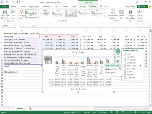
. In Excel 2013 click Design Add Chart Element Data Table to select With Legend Keys. Click the Add button. Select Show Legend at Right.

If the legend now has lots of white space select it and drag the legend corner points reduce its height to get the legend items stay closer together. In the Select Data Source dialog box under Legend Entries Series select the legend entry that you want to change and click the Edit button which resides above the list of the legend entries. To hide the data table click None.

Select an entry in the Legend Entries Series list and click Edit. In the mini toolbar in the data take menu you clicked the with legend keys menu item. The ca it refers to LDocking DockingBottom.

For more examples related to the two-variable data table of Excel click the hyperlink given before step 1 of this example. Or if the chart is on a worksheet use cells to make the table yourself. Add legend to an Excel chart.

Click Chart Filters next to the chart and click Select Data. Click the Chart Elements button and click the Chart Titles check box. Each specific entry in the legend includes a legend key for referencing the data.

From the Legend drop-down menu select the position we prefer for the legend. Now the data table is added in the chart. Legends in excel chart Legends In Excel Chart Excel chart legends depict description of significant elements and provides easy access to any chart.

The legend will then appear in the right side of the graph. A data table displays at the bottom of the chart showing the actual values. The legend is linked to the data being graphically displayed in the plot area of the chart.

These legends are represented with the help of colours or symbols and distinguish data for better understanding. Legend will appear automatically when we insert a chart in excel. Click and drag cells B2B4.

On the Chart Tools Design tab in the Data group click the Select Data button. Be careful not to select the legends color box for the entry because then youll delete the data series. Click the legend then click the top legend label and hit the Delete key.

Legend L chart1Legends1. In the Series Name field type a new legend entry. Data tables can be added to.

I am showing the values as chart labels in the chart. Not sure how your data is arrangeorganised but you could filter data to show only Greater than or equal to 0 zero such would hide the rows with NA and would display a chart with only data with value. Click cell B1 to enter it in the Series name box.

You can then select where to place the legend. Click in the Series values box and delete the default entry. In the Select Data Source dialog.

Expands or collapses the entire list. Display the data labels on this chart below the data. Select the Show Data Table option.

To quickly remove a data table from a chart you can select it and then press DELETE. Legend is the space located on the plotted area of the chart in excel. By default legends are placed to the right of the chart.

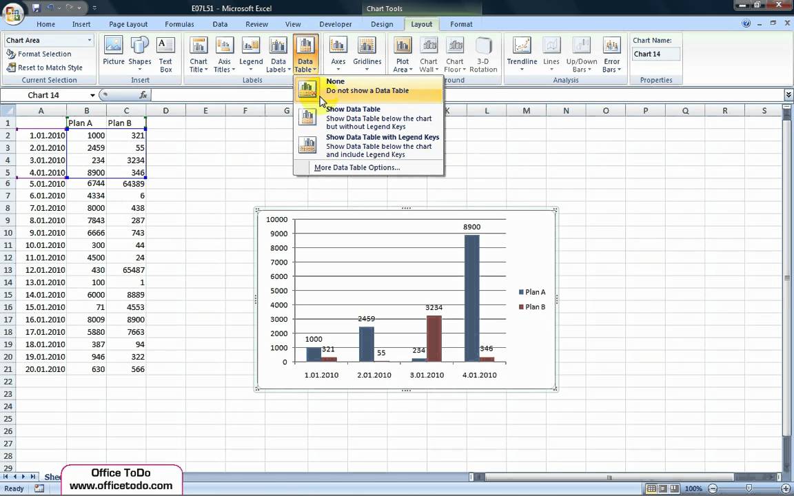
Moves to the previous or next markup in the list. Click anywhere on the chart. To display a data table click Show Data Table or Show Data Table with Legend Keys.

Read more are basically representation of data itself it is used to avoid any sorts of confusion when the data. Do one of the following. Each legend key is a graphic that visually links a legend entry with its associated series or trendline in the chart.

Make a Data Table selection. Click Layout Data Table and select Show Data Table or Show Data Table with Legend Keys option as you need. If youre only plotting one row of data then the legend isnt needed and can be deleted.

To add a data table to your selected chart and position and format it click the Chart Elements button next to the chart and then select the Data Table check box. In a chart or graph in a spreadsheet program such as Microsoft Excel the legend is often located on the right-hand side of the chart or graph and is sometimes surrounded by a border. In reply to jackie crs post on February 24 2012.

I am working a Bell Curve chart and need to insert the data table with legend in excel 2016. The Markups list toolbar contains tools for organizing processing importing and exporting data. Next we do some positioning.

The important points related to data tables of Excel are listed as follows. To add a legend to a chart select the chart then from the Design tab in the ribbon select Add Chart Element and Legend. Right-click the legend and choose Select Data in the context menu.

However each graph only needs 3-4 elements out of the 20 legend entries in the graph. Click on the data chart you want to show its data table to show the Chart Tools group in the Ribbon. If you only want certain items you will either have to use another chart placed behind the orignal one and use that to simple display the data table part.

Click Chart Tools Layout Labels Data Table. Click the Layout tab then Legend. Click the Identify Cell icon.

You can also select a cell from which the text is retrieved. You can not remove items from the Data table. In Excel 2013 click Design Add Chart Element Data Table to select With Legend Keys or No Legend Keys.

Filter and Clear Filters. Display the data table including the legend keys you launched the chart elements menu. The Key Points Governing Data Tables in Excel.

I have searched and found where one can select the layout option in the chart tools however I do not have that selection nor is it in the customize ribbon option. Bell Curve - Show Data Table with legend keys. It has Legend keys that are connected to the data source.

The legend key is linked to its associated series or trendline in such a way that changing the formatting of one simultaneously changes the formatting of the other. We can move the Legend to the top bottom right and left of the chart as per requirements by clicking on the symbol and select the Legend option drop down and choose a required. Now the data table is added in the chart.

It helps select those input values that fit the business in the best possible manner. Expand All and Collapse All. But now I want to show the data table with legend keys in the chart like it happens in excel.

How do you display the data labels on this chart below the data markers. Options include a choice not to show a data table show a data table but not show a chart legend or to show a data table and include the chart legend. On the Layout tab in the Labels group click Data Table.

How To Show Add Data Table In Chart In Excel